By Bruno Ferrari | March 26, 2020
Objective
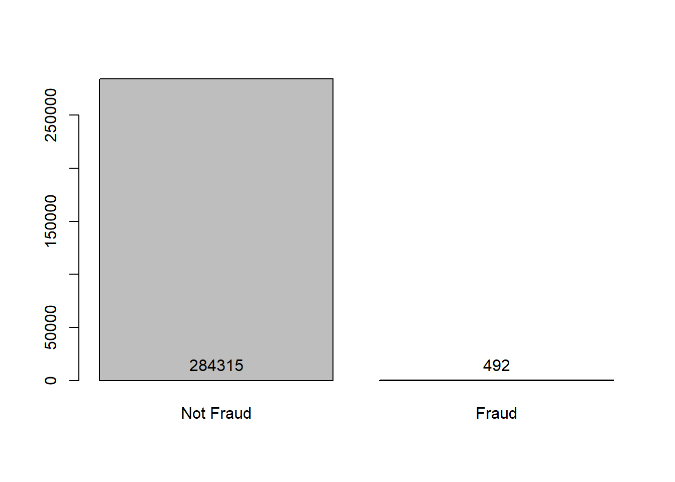
Our goal is to train a Neural Network to detect fraudulent credit card transactions in a dataset referring to two days transactions by european cardholders.
Data
credit = read.csv(path)The datasets contains transactions made by credit cards in September 2013 by european cardholders. This dataset presents transactions that occurred in two days.
As we can see, this dataset consists of thirty explanatory variables, and a response variable which represents whether a transation was a fraud or not. Due to confidentiality issues it contains only numerical input variables which are the result of a PCA transformation, the only variables which have not been transformed with PCA are ‘Time’ and ‘Amount’ (this time variable is not relevant for us, because is only a marker the transations that happened first).
str(credit)
## 'data.frame':    284807 obs. of  31 variables:
##  $ Time  : num  0 0 1 1 2 2 4 7 7 9 ...
##  $ V1    : num  -1.36 1.192 -1.358 -0.966 -1.158 ...
##  $ V2    : num  -0.0728 0.2662 -1.3402 -0.1852 0.8777 ...
##  $ V3    : num  2.536 0.166 1.773 1.793 1.549 ...
##  $ V4    : num  1.378 0.448 0.38 -0.863 0.403 ...
##  $ V5    : num  -0.3383 0.06 -0.5032 -0.0103 -0.4072 ...
##  $ V6    : num  0.4624 -0.0824 1.8005 1.2472 0.0959 ...
##  $ V7    : num  0.2396 -0.0788 0.7915 0.2376 0.5929 ...
##  $ V8    : num  0.0987 0.0851 0.2477 0.3774 -0.2705 ...
##  $ V9    : num  0.364 -0.255 -1.515 -1.387 0.818 ...
##  $ V10   : num  0.0908 -0.167 0.2076 -0.055 0.7531 ...
##  $ V11   : num  -0.552 1.613 0.625 -0.226 -0.823 ...
##  $ V12   : num  -0.6178 1.0652 0.0661 0.1782 0.5382 ...
##  $ V13   : num  -0.991 0.489 0.717 0.508 1.346 ...
##  $ V14   : num  -0.311 -0.144 -0.166 -0.288 -1.12 ...
##  $ V15   : num  1.468 0.636 2.346 -0.631 0.175 ...
##  $ V16   : num  -0.47 0.464 -2.89 -1.06 -0.451 ...
##  $ V17   : num  0.208 -0.115 1.11 -0.684 -0.237 ...
##  $ V18   : num  0.0258 -0.1834 -0.1214 1.9658 -0.0382 ...
##  $ V19   : num  0.404 -0.146 -2.262 -1.233 0.803 ...
##  $ V20   : num  0.2514 -0.0691 0.525 -0.208 0.4085 ...
##  $ V21   : num  -0.01831 -0.22578 0.248 -0.1083 -0.00943 ...
##  $ V22   : num  0.27784 -0.63867 0.77168 0.00527 0.79828 ...
##  $ V23   : num  -0.11 0.101 0.909 -0.19 -0.137 ...
##  $ V24   : num  0.0669 -0.3398 -0.6893 -1.1756 0.1413 ...
##  $ V25   : num  0.129 0.167 -0.328 0.647 -0.206 ...
##  $ V26   : num  -0.189 0.126 -0.139 -0.222 0.502 ...
##  $ V27   : num  0.13356 -0.00898 -0.05535 0.06272 0.21942 ...
##  $ V28   : num  -0.0211 0.0147 -0.0598 0.0615 0.2152 ...
##  $ Amount: num  149.62 2.69 378.66 123.5 69.99 ...
##  $ Class : int  0 0 0 0 0 0 0 0 0 0 ...
Other aspect of this dataset is that it has a highly unbalanced classes, the positive class (frauds) account for 0.172% of all transactions.
Exploiting the fact of what PCA has already been applied to data, we can makes some visual inspect of the data. If we remember the characteristics PCA technique, we have the fact which the firsts components can be used to summarize of the dataset.
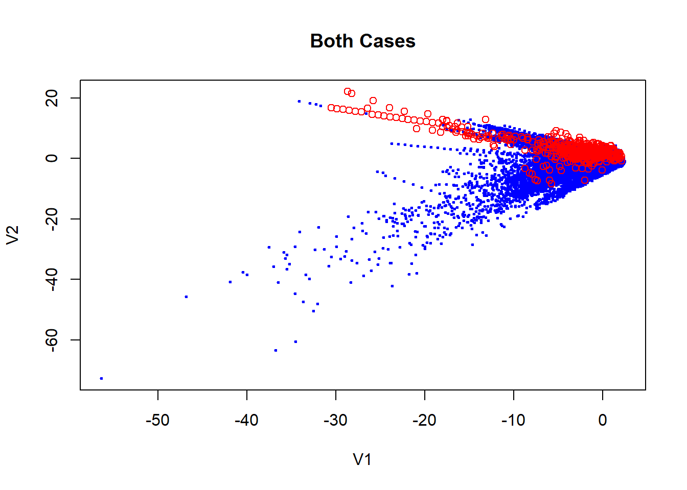
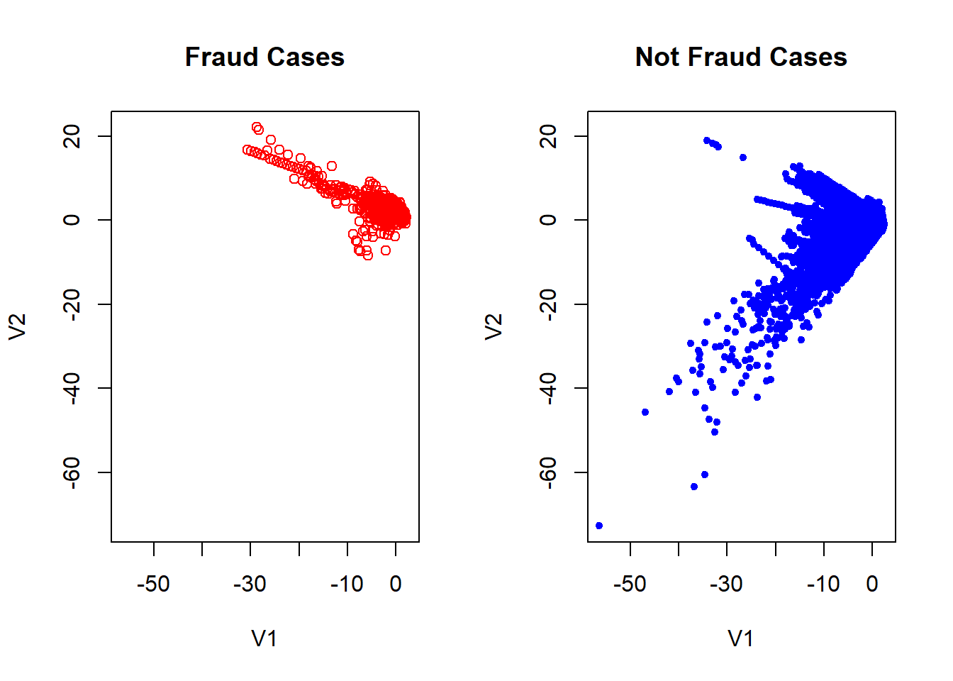
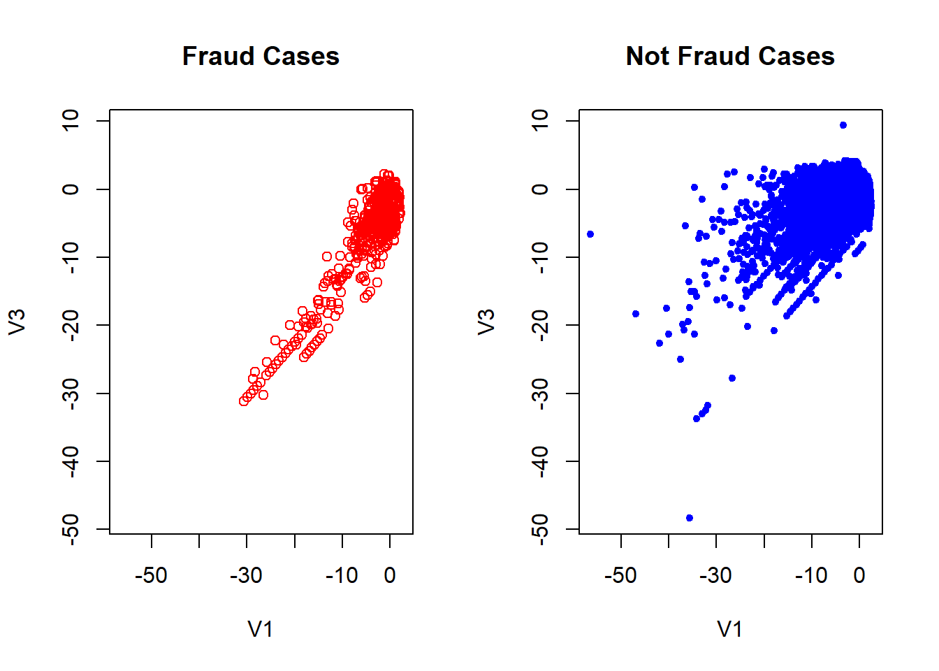
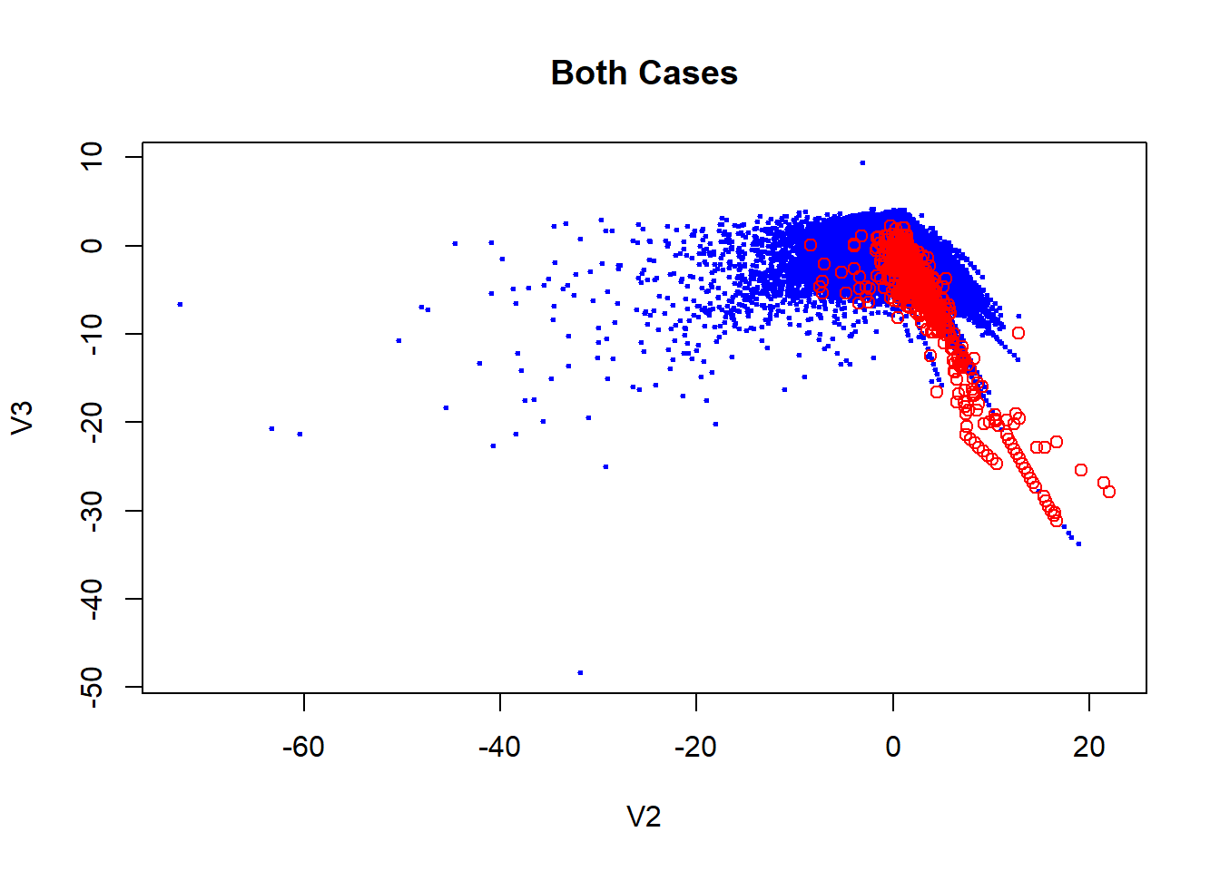
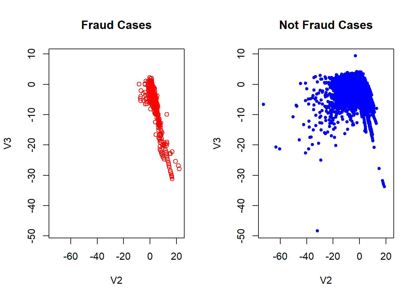
Although we don’t have the original data, it is possible to know how much of the data is explained by these components. This amount is around a 28.84% as we see blow.
credit_2 = credit[, -c(1,30,31)]
pca_credit = prcomp(credit_2)
summary(pca_credit)
## Importance of components:
## PC1 PC2 PC3 PC4 PC5 PC6
## Standard deviation 1.9587 1.65131 1.51626 1.41587 1.38025 1.33227
## Proportion of Variance 0.1248 0.08873 0.07481 0.06523 0.06199 0.05776
## Cumulative Proportion 0.1248 0.21357 0.28838 0.35361 0.41560 0.47335
## PC7 PC8 PC9 PC10 PC11 PC12
## Standard deviation 1.2371 1.19435 1.09863 1.08885 1.0207 0.99920
## Proportion of Variance 0.0498 0.04642 0.03927 0.03858 0.0339 0.03249
## Cumulative Proportion 0.5232 0.56957 0.60884 0.64742 0.6813 0.71381
## PC13 PC14 PC15 PC16 PC17 PC18
## Standard deviation 0.99527 0.9586 0.91532 0.87625 0.84934 0.83818
## Proportion of Variance 0.03223 0.0299 0.02726 0.02498 0.02347 0.02286
## Cumulative Proportion 0.74605 0.7760 0.80321 0.82819 0.85167 0.87453
## PC19 PC20 PC21 PC22 PC23 PC24
## Standard deviation 0.81404 0.77093 0.73452 0.72570 0.62446 0.60565
## Proportion of Variance 0.02156 0.01934 0.01756 0.01714 0.01269 0.01194
## Cumulative Proportion 0.89609 0.91543 0.93298 0.95012 0.96281 0.97474
## PC25 PC26 PC27 PC28
## Standard deviation 0.52128 0.48223 0.4036 0.33008
## Proportion of Variance 0.00884 0.00757 0.0053 0.00355
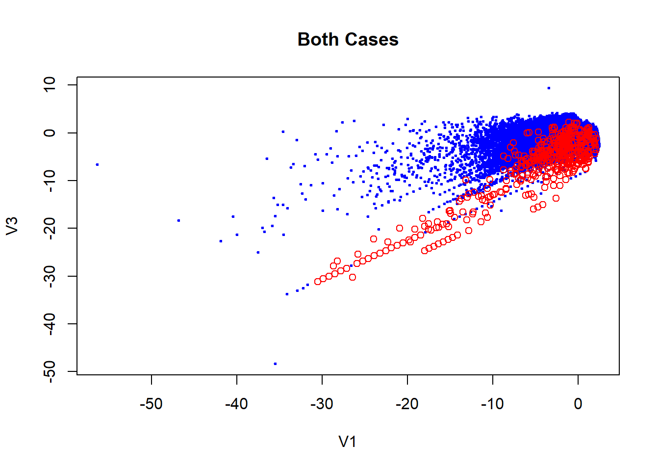
## Cumulative Proportion 0.98359 0.99115 0.9964 1.00000Here we can see how the fraudulent transactions and the not fraudulent in general is quite similar. In the plot is actually true which there are some red cases which separate of the blues one but considering how unbalanced is the data, this can be not representative. This makes our job harder because is not clear what characteristics makes a fraudulent transactions.
Model Fitting
As discussed above, we have two main caracteristics of the data:
1 High unbalanced classes
2 Homogeneity our not cleary separations of the classes at least in low dimensions.
So, because of that, we going to use a Neural Network to indentify fraud transactions. Neural Networks have huge capacities in sense to adapt well in many raw data and therefore not need (in general) does data transformations. This is important because we do not have access to original data.
Packages used in this job.
library("caTools")
library("caret")
library("keras")
library("ROCR")
Continuing, let splitting the dataset into train and test. We also going to drop-off the time features of the dataset.
credit = credit[, -c(1)]

set.seed(42)

split = sample.split(credit$Class, SplitRatio = 0.75)
train = subset(credit, split==TRUE)
test = subset(credit, split==FALSE)
Using the keras package we create our Neural Network with 29 input layer (dimension of the dataset), one hidden layer with 32 neurons and 1 neuron on output layer.
model <- keras_model_sequential(name = "credit_NN")
model %>%
  layer_dense(units = 32, activation = 'relu', input_shape = 29, kernel_initializer = 'uniform', name = "NN_IN") %>%
  layer_dense(units = 1 , activation = 'sigmoid', kernel_initializer = 'uniform', name = "NN_OUT")
model
## Model
## Model: "credit_NN"
## ___________________________________________________________________________
## Layer (type)                     Output Shape                  Param #
## ===========================================================================
## NN_IN (Dense)                    (None, 32)                    960
## ___________________________________________________________________________
## NN_OUT (Dense)                   (None, 1)                     33
## ===========================================================================
## Total params: 993
## Trainable params: 993
## Non-trainable params: 0
## ___________________________________________________________________________
Compile the Network, and choose the accuracy metric for evaluation.
model %>% compile(
  loss = 'binary_crossentropy',
  optimizer = "adam",
  metrics = c('accuracy')
)
Fitting the Network with the data.
history <- model %>% fit(
  x = as.matrix(train[, -c(30)]), y = train[, c(30)],
  epochs = 30, batch_size = 128,
  validation_split = 0.2
)

plot(history)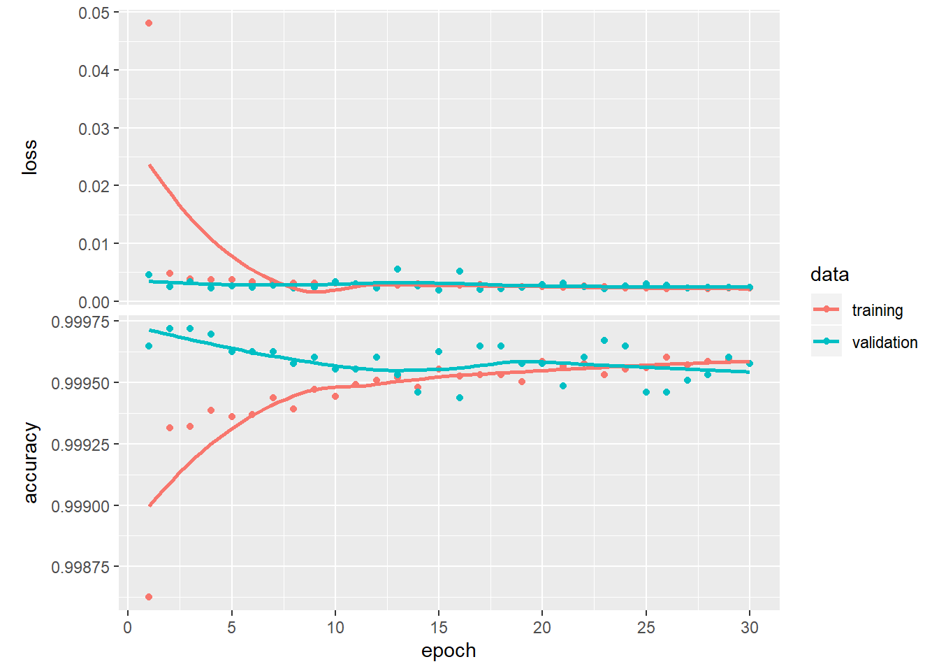
Results
For evaluate how good our network are, we going to set a dummy model which predict that all results is the main class (0 - Not Fraud). As we see below, the accuracy of this model is around of 99.83%, so is desirable our Neural Network has better results.
y_dummy = replicate(nrow(credit), 0)

confusionMatrix(data = as.factor(y_dummy), reference = as.factor(credit$Class), positive = "1", mode = "prec_recall")
## Confusion Matrix and Statistics
##
##           Reference
## Prediction      0      1
##          0 284315    492
##          1      0      0
##
##                Accuracy : 0.9983
##                  95% CI : (0.9981, 0.9984)
##     No Information Rate : 0.9983
##     P-Value [Acc > NIR] : 0.512
##
##                   Kappa : 0
##
##  Mcnemar's Test P-Value : <2e-16
##
##               Precision :       NA
##                  Recall : 0.000000
##                      F1 :       NA
##              Prevalence : 0.001727
##          Detection Rate : 0.000000
##    Detection Prevalence : 0.000000
##       Balanced Accuracy : 0.500000
##
##        'Positive' Class : 1
##
Here we can see the results of our model, which has a 99,94% of accuracy, slightly above of the dummy model but other statics are also important, such as a Recall rate which measures how well the model can correctly forecast the fraud class, which is our main objective. Considering again how unballanced are the class, we have here a good rate high than 70%
y_pred = model %>% predict_classes(as.matrix(test[,-c(30)]))
confusionMatrix(as.factor(y_pred), as.factor(test$Class), mode = "prec_recall", positive = "1")
## Confusion Matrix and Statistics
##
##           Reference
## Prediction     0     1
##          0 71068    29
##          1    11    94
##
##                Accuracy : 0.9994
##                  95% CI : (0.9992, 0.9996)
##     No Information Rate : 0.9983
##     P-Value [Acc > NIR] : < 2e-16
##
##                   Kappa : 0.8243
##
##  Mcnemar's Test P-Value : 0.00719
##
##               Precision : 0.895238
##                  Recall : 0.764228
##                      F1 : 0.824561
##              Prevalence : 0.001727
##          Detection Rate : 0.001320
##    Detection Prevalence : 0.001475
##       Balanced Accuracy : 0.882036
##
##        'Positive' Class : 1
##
Other metric which measures how well is the model is the AUC (Area under the Curve) of ROC (Receiver Operating Characteristic) Curve. 0.7 to 0.8 is considered acceptable, 0.8 to 0.9 is considered excellent, and more than 0.9 is considered outstanding. The ROC curve show the tradeoff between the True Positive Rate and the False Positive Rate.
y_pred2 = model %>% predict_proba(as.matrix(test[,-c(30)]))
ROCRpred = prediction(y_pred2, test$Class)
ROCRperf = performance(ROCRpred, "tpr", "fpr")
auc_ROCR = performance(ROCRpred, measure = "auc")
auc_ROCR = auc_ROCR@y.values[[1]]
plot(ROCRperf, colorize=TRUE)
legend(0.8, 0.2, legend=c("AUC Area:", round(auc_ROCR, 2)), cex=0.8)
abline(a = 0, b = 1)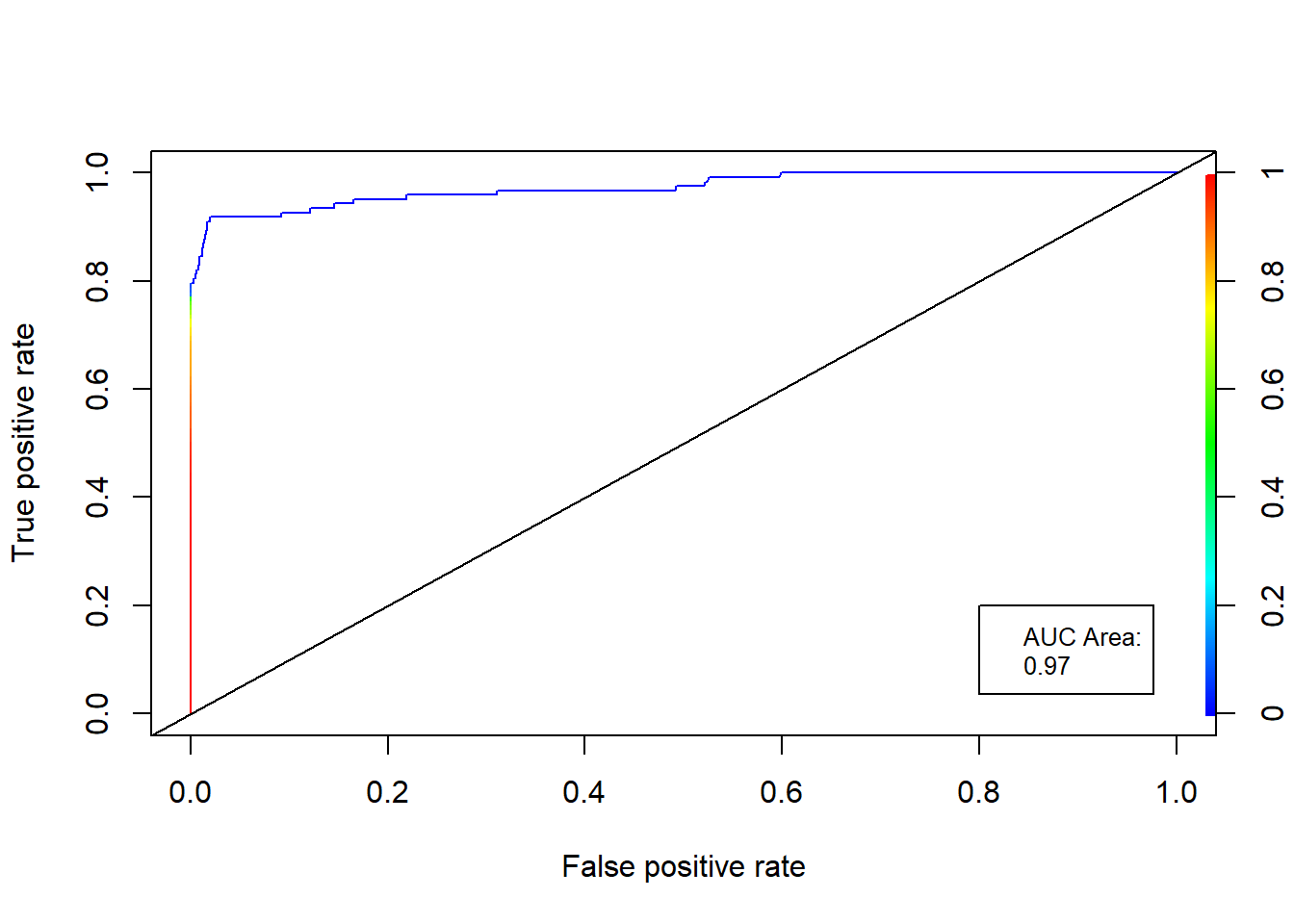
Conclusions
We can observe that Neural Networks are powerful structures. Although the highly unbalanced classes, no tunning of the model hyperparameters, and any data manipulations, The generated model shows good results identifying the fraud transactions of the dataset.