By Salerno | March 18, 2020
1. The Iris dataset in scikit-learn
from sklearn import datasets
import pandas as pd
import numpy as np
import matplotlib.pyplot as plt

plt.style.use('ggplot')
iris = datasets.load_iris()
type(iris)
## <class 'sklearn.utils.Bunch'>
print(iris.keys())## dict_keys(['data', 'target', 'target_names', 'DESCR', 'feature_names', 'filename'])print(iris.DESCR)
## .. _iris_dataset:
##
## Iris plants dataset
## --------------------
##
## **Data Set Characteristics:**
##
##     :Number of Instances: 150 (50 in each of three classes)
##     :Number of Attributes: 4 numeric, predictive attributes and the class
##     :Attribute Information:
##         - sepal length in cm
##         - sepal width in cm
##         - petal length in cm
##         - petal width in cm
##         - class:
##                 - Iris-Setosa
##                 - Iris-Versicolour
##                 - Iris-Virginica
##
##     :Summary Statistics:
##
##     ============== ==== ==== ======= ===== ====================
##                     Min  Max   Mean    SD   Class Correlation
##     ============== ==== ==== ======= ===== ====================
##     sepal length:   4.3  7.9   5.84   0.83    0.7826
##     sepal width:    2.0  4.4   3.05   0.43   -0.4194
##     petal length:   1.0  6.9   3.76   1.76    0.9490  (high!)
##     petal width:    0.1  2.5   1.20   0.76    0.9565  (high!)
##     ============== ==== ==== ======= ===== ====================
##
##     :Missing Attribute Values: None
##     :Class Distribution: 33.3% for each of 3 classes.
##     :Creator: R.A. Fisher
##     :Donor: Michael Marshall (MARSHALL%PLU@io.arc.nasa.gov)
##     :Date: July, 1988
##
## The famous Iris database, first used by Sir R.A. Fisher. The dataset is taken
## from Fisher's paper. Note that it's the same as in R, but not as in the UCI
## Machine Learning Repository, which has two wrong data points.
##
## This is perhaps the best known database to be found in the
## pattern recognition literature.  Fisher's paper is a classic in the field and
## is referenced frequently to this day.  (See Duda & Hart, for example.)  The
## data set contains 3 classes of 50 instances each, where each class refers to a
## type of iris plant.  One class is linearly separable from the other 2; the
## latter are NOT linearly separable from each other.
##
## .. topic:: References
##
##    - Fisher, R.A. "The use of multiple measurements in taxonomic problems"
##      Annual Eugenics, 7, Part II, 179-188 (1936); also in "Contributions to
##      Mathematical Statistics" (John Wiley, NY, 1950).
##    - Duda, R.O., & Hart, P.E. (1973) Pattern Classification and Scene Analysis.
##      (Q327.D83) John Wiley & Sons.  ISBN 0-471-22361-1.  See page 218.
##    - Dasarathy, B.V. (1980) "Nosing Around the Neighborhood: A New System
##      Structure and Classification Rule for Recognition in Partially Exposed
##      Environments".  IEEE Transactions on Pattern Analysis and Machine
##      Intelligence, Vol. PAMI-2, No. 1, 67-71.
##    - Gates, G.W. (1972) "The Reduced Nearest Neighbor Rule".  IEEE Transactions
##      on Information Theory, May 1972, 431-433.
##    - See also: 1988 MLC Proceedings, 54-64.  Cheeseman et al"s AUTOCLASS II
##      conceptual clustering system finds 3 classes in the data.
##    - Many, many more ...
type(iris.data), type(iris.target)## (<class 'numpy.ndarray'>, <class 'numpy.ndarray'>)
iris.data.shape## (150, 4)
iris.target_names## array(['setosa', 'versicolor', 'virginica'], dtype='<U10')2. Exploratory data analysis (EDA)
X = iris.data
y = iris.target
df = pd.DataFrame(X, columns=iris.feature_names)
print(df.head())
## sepal length (cm) sepal width (cm) petal length (cm) petal width (cm)
## 0 5.1 3.5 1.4 0.2
## 1 4.9 3.0 1.4 0.2
## 2 4.7 3.2 1.3 0.2
## 3 4.6 3.1 1.5 0.2
## 4 5.0 3.6 1.4 0.23. Visual EDA
_ = pd.plotting.scatter_matrix(df, c = y, figsize = [8, 8],
s=150, marker = 'D')
plt.savefig('./_bookdown_files/_main_files/figure-html/iris.png')
plt.show()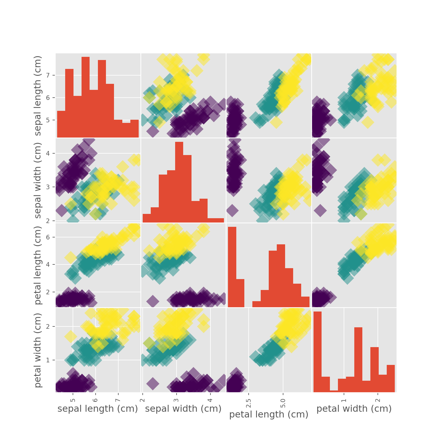
4. Using scikit-learn to fit a classifier
from sklearn.neighbors import KNeighborsClassifier

knn = KNeighborsClassifier(n_neighbors=6)

X = iris['data']
y = iris['target']

# Fit the classifier to the data
knn.fit(X, y)
## KNeighborsClassifier(algorithm='auto', leaf_size=30, metric='minkowski',
## metric_params=None, n_jobs=None, n_neighbors=6, p=2,
## weights='uniform')X.shape## (150, 4)y.shape## (150,)5. Predicting on unlabeled data
# Predict the labels for the training data X
y_pred = knn.predict(X)
print("Prediction: {}".format(y_pred))## Prediction: [0 0 0 0 0 0 0 0 0 0 0 0 0 0 0 0 0 0 0 0 0 0 0 0 0 0 0 0 0 0 0 0 0 0 0 0 0
## 0 0 0 0 0 0 0 0 0 0 0 0 0 1 1 1 1 1 1 1 1 1 1 1 1 1 1 1 1 1 1 1 1 1 1 2 1
## 1 1 1 1 1 1 1 1 1 2 1 1 1 1 1 1 1 1 1 1 1 1 1 1 1 1 2 2 2 2 2 2 1 2 2 2 2
## 2 2 2 2 2 2 2 2 1 2 2 2 2 2 2 2 2 2 2 2 2 2 2 2 2 2 2 2 2 2 2 2 2 2 2 2 2
## 2 2]6. Train/Test split
from sklearn.model_selection import train_test_split
X_train, X_test, y_train, y_test = train_test_split(X, y, test_size=0.3, random_state=21, stratify=y)
knn = KNeighborsClassifier(n_neighbors=8)
knn.fit(X_train, y_train)## KNeighborsClassifier(algorithm='auto', leaf_size=30, metric='minkowski',
## metric_params=None, n_jobs=None, n_neighbors=8, p=2,
## weights='uniform')y_pred = knn.predict(X_test)
print("Test set predictions:\n", "{}".format(y_pred))## Test set predictions:
## [2 1 2 2 1 0 1 0 0 1 0 2 0 2 2 0 0 0 1 0 2 2 2 0 1 1 1 0 0 1 2 2 0 0 1 2 2
## 1 1 2 1 1 0 2 1]
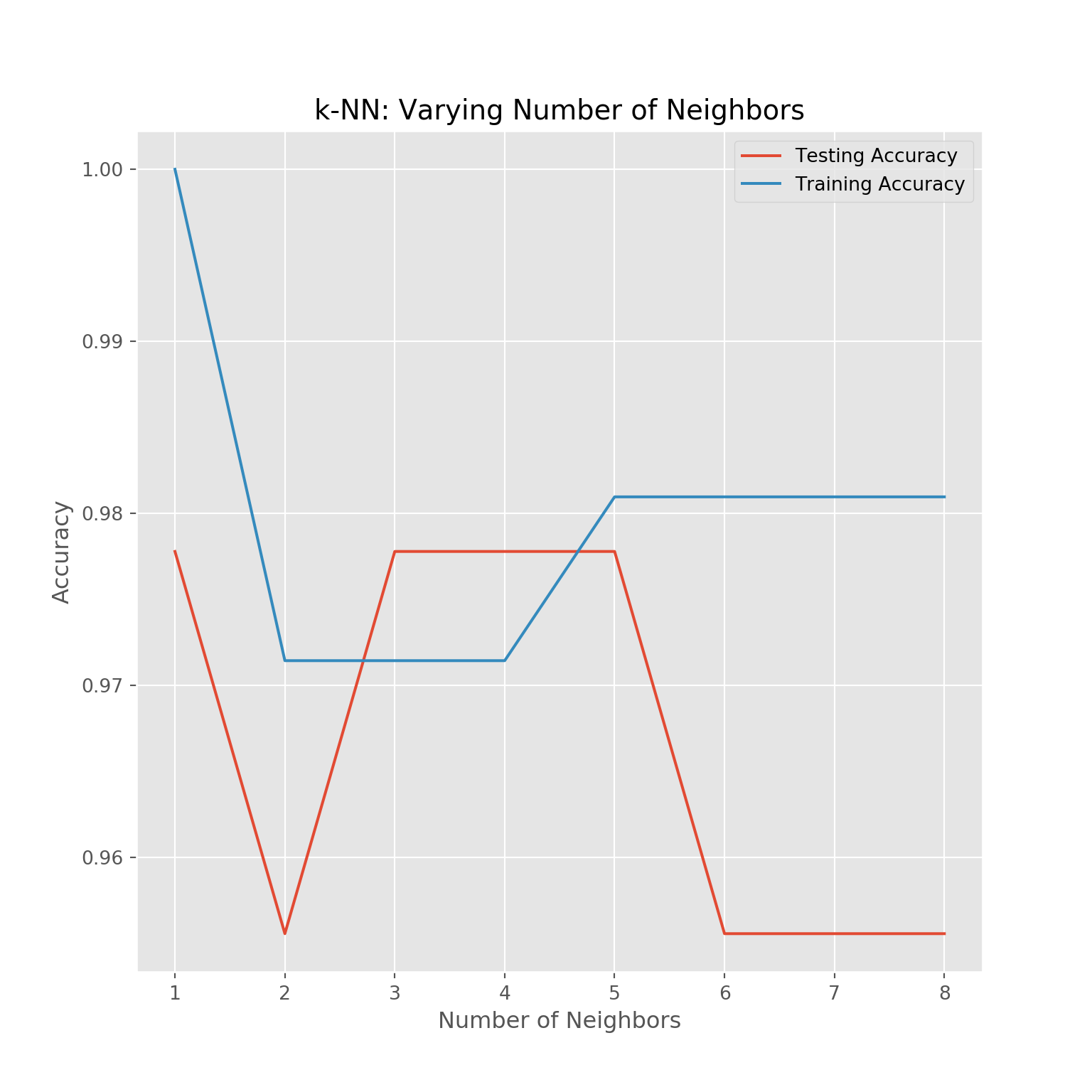
knn.score(X_test, y_test)## 0.95555555555555567. Overfitting and underfitting
# Setup arrays to store train and test accuracies
neighbors = np.arange(1, 9)
train_accuracy = np.empty(len(neighbors))
test_accuracy = np.empty(len(neighbors))
# Loop over different values of k
for i, k in enumerate(neighbors):
# Setup a k-NN Classifier with k neighbors: knn
knn = KNeighborsClassifier(n_neighbors=k)
# Fit the classifier to the training data
knn.fit(X_train, y_train)
#Compute accuracy on the training set
train_accuracy[i] = knn.score(X_train, y_train)
#Compute accuracy on the testing set
test_accuracy[i] = knn.score(X_test, y_test)
# Generate plot## KNeighborsClassifier(algorithm='auto', leaf_size=30, metric='minkowski',
## metric_params=None, n_jobs=None, n_neighbors=1, p=2,
## weights='uniform')
## KNeighborsClassifier(algorithm='auto', leaf_size=30, metric='minkowski',
## metric_params=None, n_jobs=None, n_neighbors=2, p=2,
## weights='uniform')
## KNeighborsClassifier(algorithm='auto', leaf_size=30, metric='minkowski',
## metric_params=None, n_jobs=None, n_neighbors=3, p=2,
## weights='uniform')
## KNeighborsClassifier(algorithm='auto', leaf_size=30, metric='minkowski',
## metric_params=None, n_jobs=None, n_neighbors=4, p=2,
## weights='uniform')
## KNeighborsClassifier(algorithm='auto', leaf_size=30, metric='minkowski',
## metric_params=None, n_jobs=None, n_neighbors=5, p=2,
## weights='uniform')
## KNeighborsClassifier(algorithm='auto', leaf_size=30, metric='minkowski',
##                      metric_params=None, n_jobs=None, n_neighbors=6, p=2,
##                      weights='uniform')
## KNeighborsClassifier(algorithm='auto', leaf_size=30, metric='minkowski',
## metric_params=None, n_jobs=None, n_neighbors=7, p=2,
## weights='uniform')
## KNeighborsClassifier(algorithm='auto', leaf_size=30, metric='minkowski',
##                      metric_params=None, n_jobs=None, n_neighbors=8, p=2,
## weights='uniform')plt.title('k-NN: Varying Number of Neighbors')## Text(0.5, 1.0, 'k-NN: Varying Number of Neighbors')plt.plot(neighbors, test_accuracy, label = 'Testing Accuracy')## [<matplotlib.lines.Line2D object at 0x000000002E750AC8>]plt.plot(neighbors, train_accuracy, label = 'Training Accuracy')## [<matplotlib.lines.Line2D object at 0x000000002E787D88>]plt.legend()## <matplotlib.legend.Legend object at 0x000000002E765448>plt.xlabel('Number of Neighbors')## Text(0.5, 0, 'Number of Neighbors')plt.ylabel('Accuracy')## Text(0, 0.5, 'Accuracy')plt.savefig('./_bookdown_files/_main_files/figure-html/knn.png')
plt.show()