Correlation and Regression

path <- "C:/Users/andre/OneDrive/Área de Trabalho/salerno/blogdown/datasets/ncbirths"

path <- paste0(path, "/ncbirths.csv")

data <- read.csv(path, stringsAsFactors = FALSE)

dim(data)
## [1] 1450   15

names(data)
##  [1] "ID"            "Plural"        "Sex"           "MomAge"       
##  [5] "Weeks"         "Marital"       "RaceMom"       "HispMom"      
##  [9] "Gained"        "Smoke"         "BirthWeightOz" "BirthWeightGm"
## [13] "Low"           "Premie"        "MomRace"

library(ggplot2)

ggplot(data = data, aes(y = BirthWeightOz, x = Weeks)) +
geom_point()
## Warning: Removed 1 rows containing missing values (geom_point).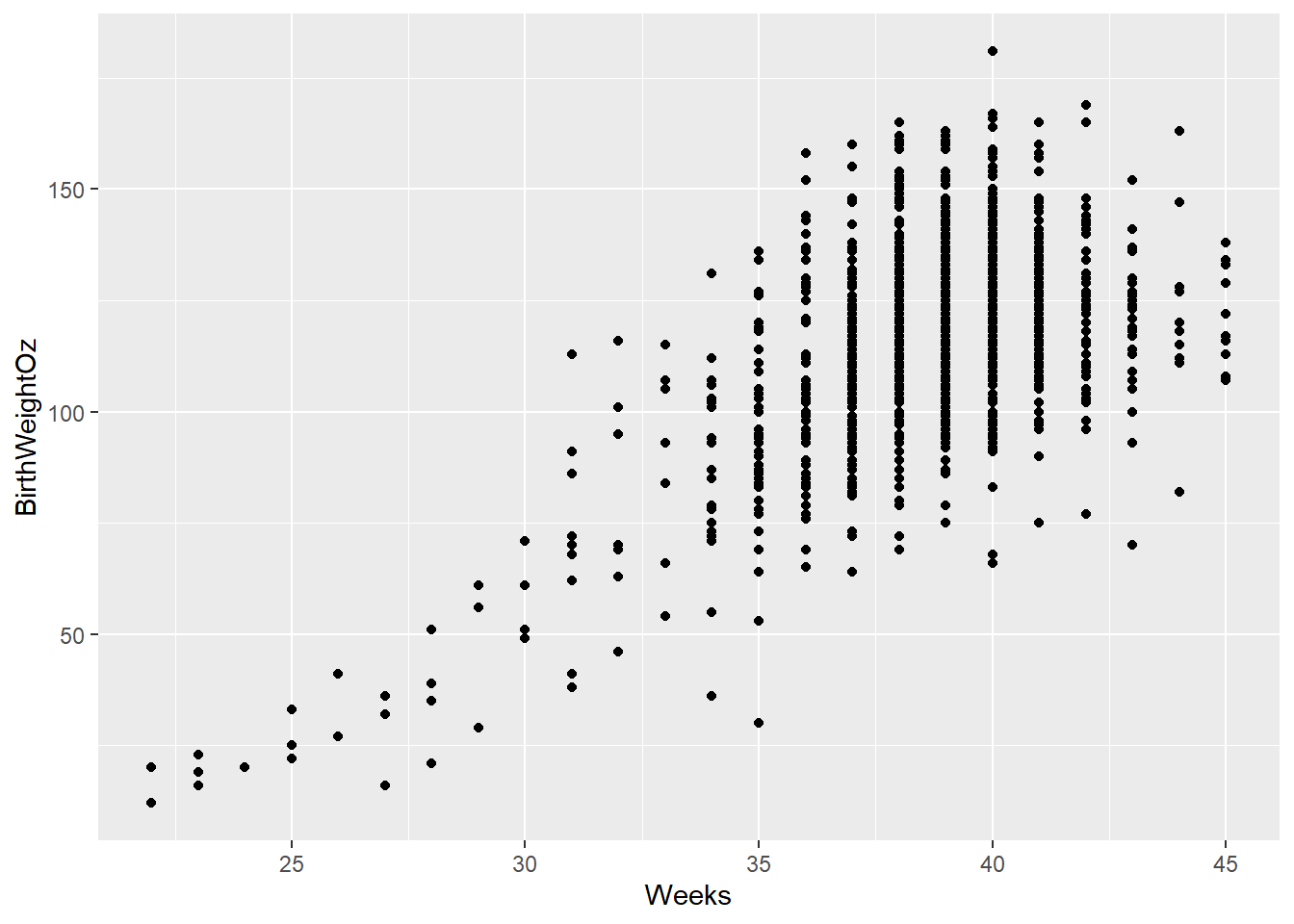

# Boxplot of weight vs. weeks
ggplot(data = data, 
       aes(x = cut(Weeks, breaks = 5), y = BirthWeightOz)) + 
  geom_boxplot()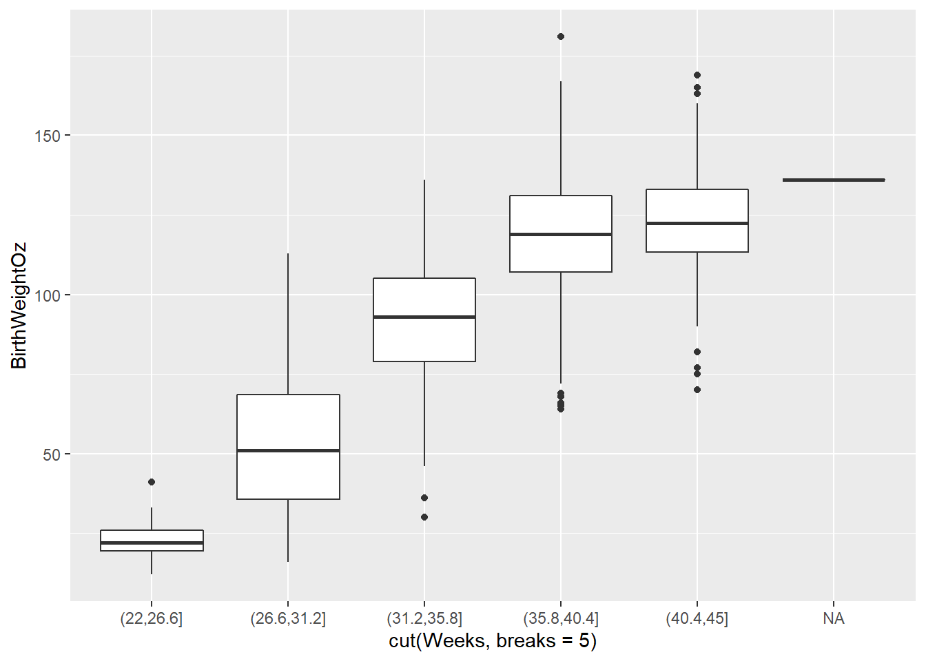

library(tidyverse)
## computing correlation

data %>%
  summarize(N = n(), r = cor(BirthWeightOz, MomAge))
##      N         r
## 1 1450 0.1461145

# Compute correlation for all non-missing pairs
data %>%
  summarize(N = n(), r = cor(BirthWeightOz, MomAge, use = "pairwise.complete.obs"))
##      N         r
## 1 1450 0.1461145

library(openintro)
## Please visit openintro.org for free statistics materials
## 
## Attaching package: 'openintro'
## The following object is masked from 'package:ggplot2':
## 
##     diamonds
## The following objects are masked from 'package:datasets':
## 
##     cars, trees

ggplot(data = mammals, aes(y = BrainWt, x = BodyWt)) +
    geom_point()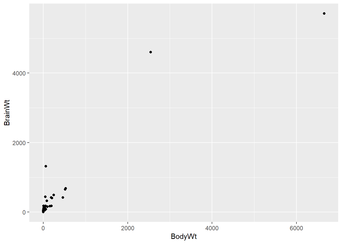

# Scatterplot with coord_trans()
ggplot(data = mammals, aes(y = BrainWt, x = BodyWt)) +
  geom_point() + 
  coord_trans(x = "log10", y = "log10")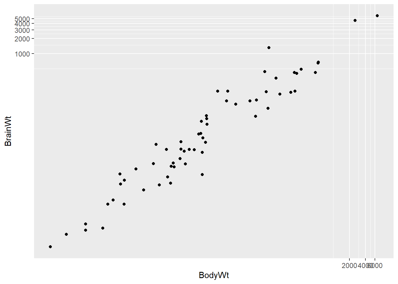

# Scatterplot with scale_x_log10() and scale_y_log10()
ggplot(data = mammals, aes(x = BodyWt, y = BrainWt)) +
  geom_point() +
  scale_x_log10() + 
  scale_y_log10()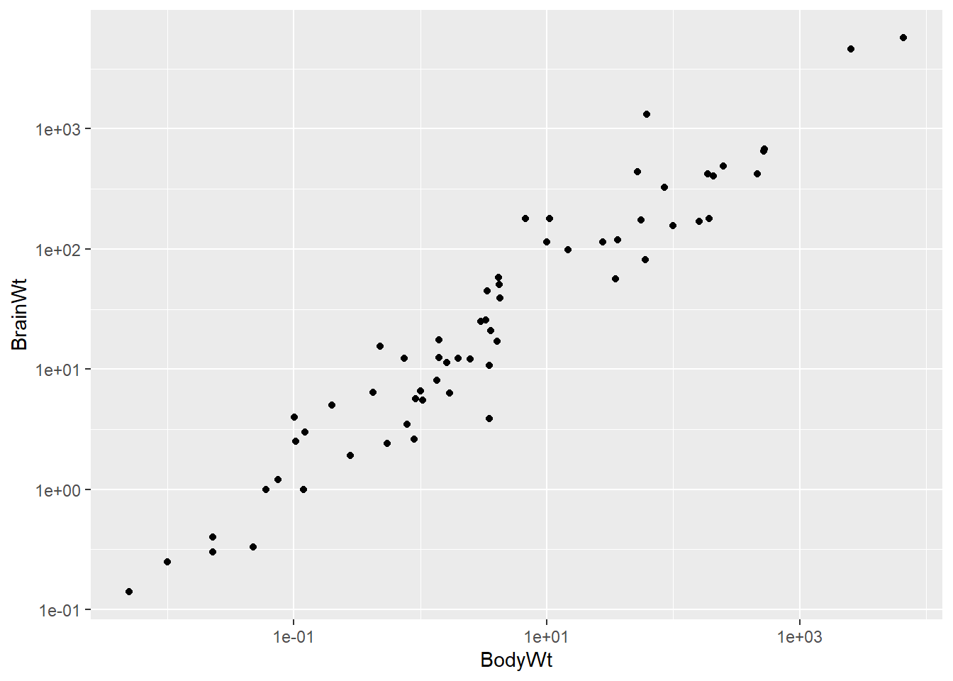

# Correlation among mammals, with and without log
mammals %>%
  summarize(N = n(), 
            r = cor(BodyWt, BrainWt), 
            r_log = cor(log(BodyWt), log(BrainWt)))
##    N         r     r_log
## 1 62 0.9341638 0.9595748

library(tidyverse)
ggplot(data = mlbBat10, aes(y = SLG, x = OBP)) +
    geom_point()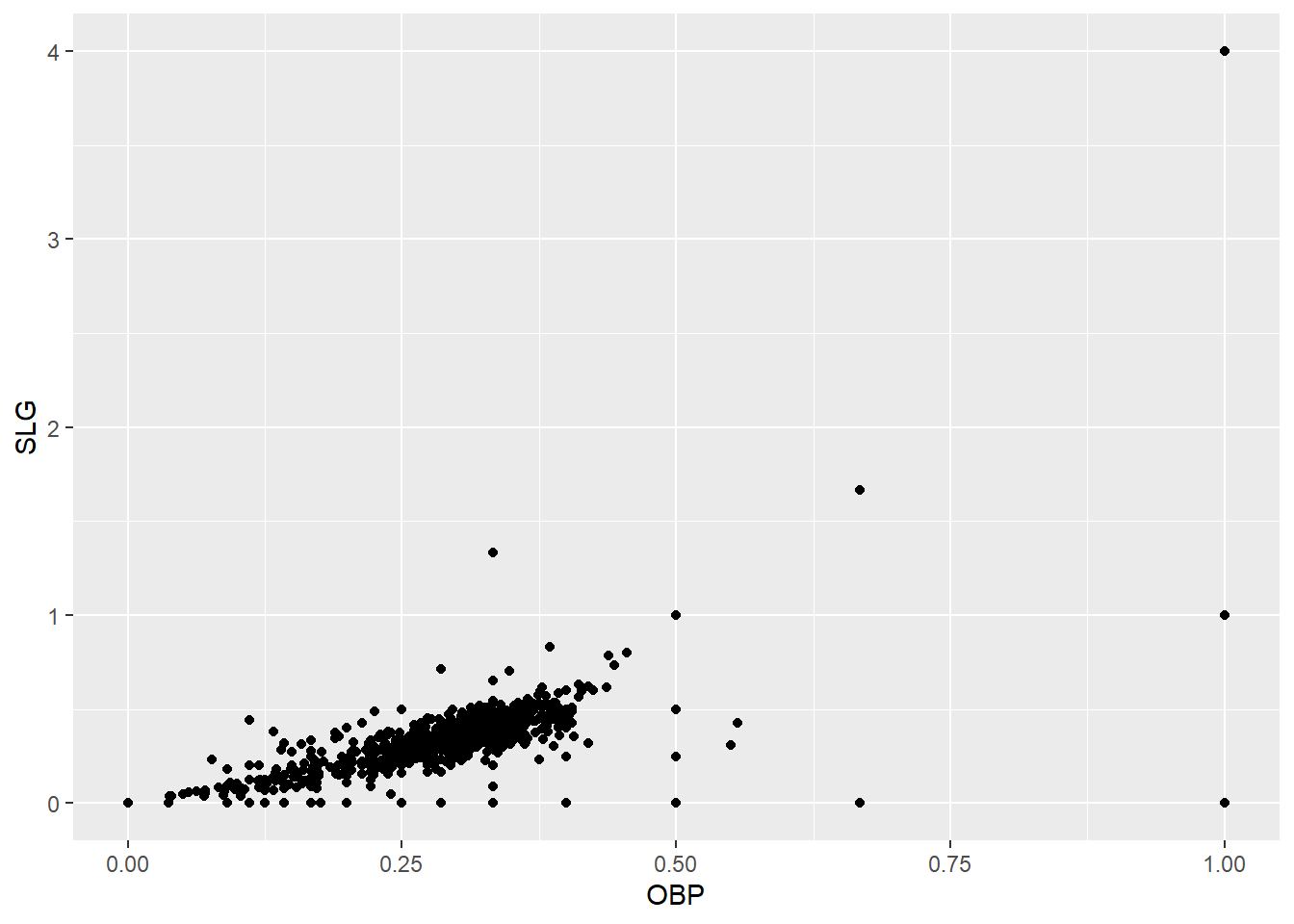

# identifying outliers
# Filter for AB greater than or equal to 200
ab_gt_200 <- mlbBat10 %>%
  filter(AB >= 200) 

# Scatterplot of SLG vs. OBP
ggplot(ab_gt_200, aes(x = OBP, y = SLG)) +
  geom_point()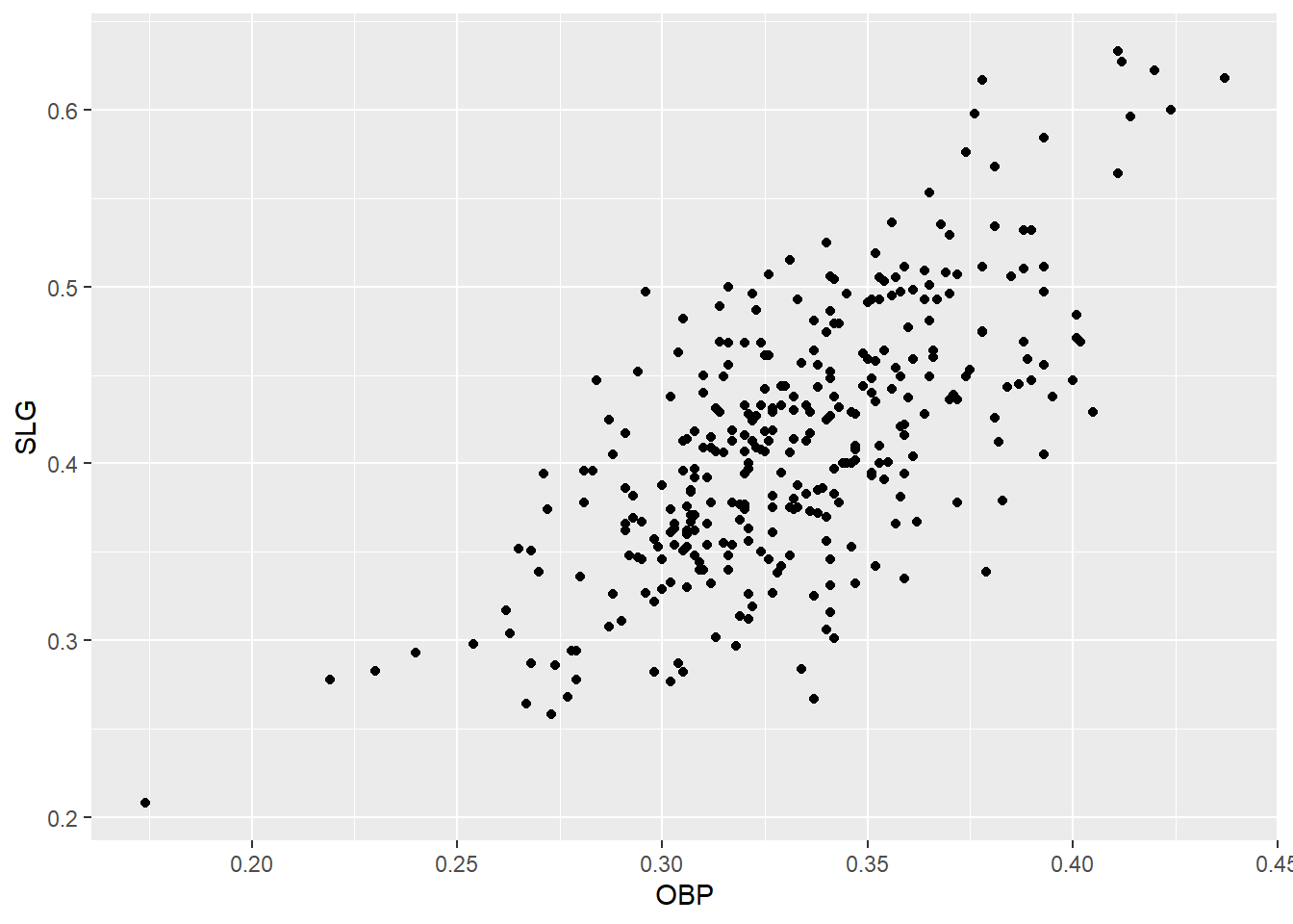

# Identify the outlying player
ab_gt_200 %>%
  filter(OBP < 0.2)
##     name team position  G  AB  R  H 2B 3B HR RBI TB BB SO SB CS   OBP   SLG
## 1 B Wood  LAA       3B 81 226 20 33  2  0  4  14 47  6 71  1  0 0.174 0.208
##     AVG
## 1 0.146

# Correlation for all baseball players
mlbBat10 %>%
  summarize(N = n(), r = cor(OBP, SLG))
##      N         r
## 1 1199 0.8145628

# Run this and look at the plot
mlbBat10 %>% 
    filter(AB > 200) %>%
    ggplot(aes(x = OBP, y = SLG)) + 
    geom_point()

# Correlation for all players with at least 200 ABs
mlbBat10 %>%
  filter(AB >= 200) %>%
  summarize(N = n(), r = cor(OBP, SLG))
##     N         r
## 1 329 0.6855364

# Run this and look at the plot
ggplot(data = bdims, aes(x = hgt, y = wgt, color = factor(sex))) +
  geom_point()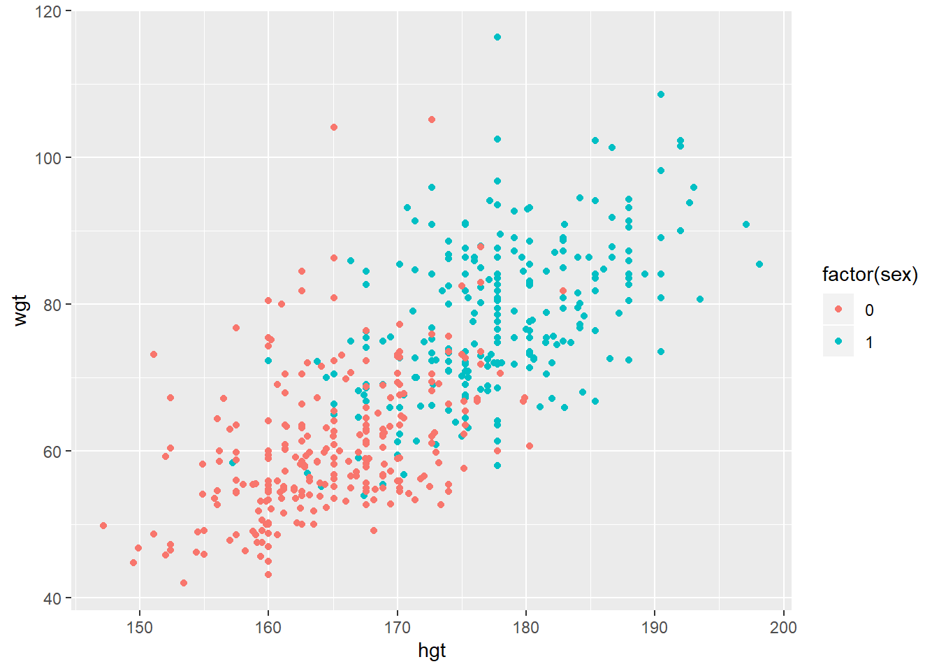 

# Correlation of body dimensions
bdims %>%
  group_by(sex) %>%
  summarize(N = n(), r = cor(hgt, wgt))
## # A tibble: 2 x 3
##     sex     N     r
##   <int> <int> <dbl>
## 1     0   260 0.431
## 2     1   247 0.535

ggplot(data = smoking, aes(y = amtWeekdays, x = age)) +
      geom_point()
## Warning: Removed 1270 rows containing missing values (geom_point).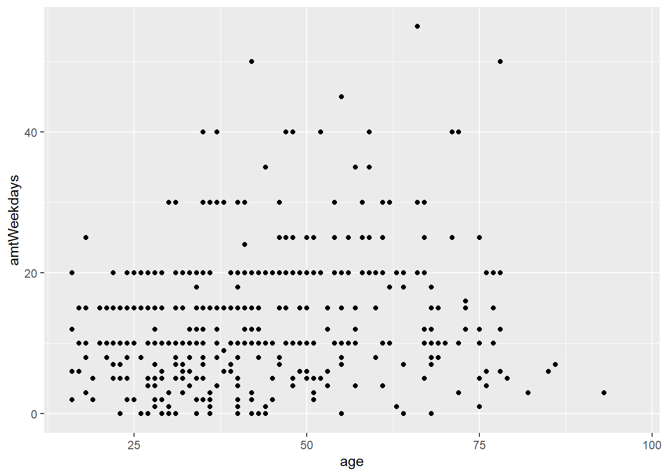

path1 <- "C:/Users/andre/OneDrive/Área de Trabalho/salerno/blogdown/datasets/anscombe"

path1 <- paste0(path1, "/anscombe.csv")

anscombe <- read.csv(path1, stringsAsFactors = FALSE, sep = ";")


# Compute properties of Anscombe
anscombe %>%
  group_by(set) %>%
  summarize(
    N = n(), 
    mean_of_x = mean(x), 
    std_dev_of_x = sd(x), 
    mean_of_y = mean(y), 
    std_dev_of_y = sd(y), 
    correlation_between_x_and_y = cor(x, y)
  )
## # A tibble: 4 x 7
##     set     N mean_of_x std_dev_of_x mean_of_y std_dev_of_y correlation_between…
##   <int> <int>     <dbl>        <dbl>     <dbl>        <dbl>                <dbl>
## 1     1    11         9         3.32      7.50         2.03                0.816
## 2     2    11         9         3.32      7.50         2.03                0.816
## 3     3    11         9         3.32      7.5          2.03                0.816
## 4     4    11         9         3.32      7.50         2.03                0.817